Defining triangulation settings
The main purpose of the Triangulation Settings step in the Seismic Interpretation workflow (prepare > Seismic > Triangulation Settings) is to define the triangulation settings for faults in your seismic interpretation.
To define the triangulation settings:
- Open the Triangulation Settings form (prepare > Seismic > Triangulation Settings) and at the top of the form, select the relevant Seismic Interpretation from the Interpretation drop-down list.
- Click the + sign in front of the Faults section to expand the column and review the data representations (the Polyline Set column shows the polyline sets available for triangulation; the Tri-mesh column shows any tri-meshes already present for the relevant faults).
- (Optional) In the Create QC Tri-mesh column, check the checkbox for faults for which you want to generate a QC tri-mesh. The generated tri-meshes will appear in your Seismic Interpretation next to the polyline set representations.
- Click the + sign at the front of the Triangulation Settings section to expand the columns and view more detail the triangulation settings.
- Choose from various Boundary Method settings for each surface. You can select a boundary method per surface, or change it for all surfaces at once. To specify a method for all surfaces, right-click in the table and select Set boundary method globally. This opens a context menu with all boundary methods.
- Select Convex hull to create a convex hull around the data points. This is generally a good method for horizons.
- Fit to data – area fit, no gaps is an algorithm that closely follows the input data and allows concave shapes but no gaps. The result is influenced by the step dimensions of the input area.
- Fit to data – tight fit is the algorithm that most closely follows the input data and allows gaps to occur. Although the most accurate as far as representing the input data is concerned, using it may be a trade-off between accuracy and the work required to produce a surface suitable for modeling. Your data will be accurately represented, but you may have to repair the surface later using the tri-mesh editing tools or, to avoid this, use a less accurate bounding method.
- Select Boundary polygon and then a 'boundary' (polyline set with a single closed polyline) from the drop-down list in the Boundary Polygon column (which lists all such polygons in your solution) to use to cut out the resulting tri-mesh. All data values generated outside the boundary will be blanked.
- Choose from various Projection Type settings for each surface. The triangulation algorithms require that polylines are projected onto a plane, and a projection vector is computed automatically for each polyline set. Sometimes it is desirable to override the default projection vector
- Select User defined and enter values for Projection Dip and Projection Azimuth.
- Select Reset to default to return to the default projection settings.
- Select Set from [View] to derive the Projection Dip and Projection Azimuth based on the orientation of the selected View.
- Click the + sign at the front of the Dimensions section to expand the column and view the Length and Height of the surface as well as its Area.
- Click Apply or OK to save your settings.
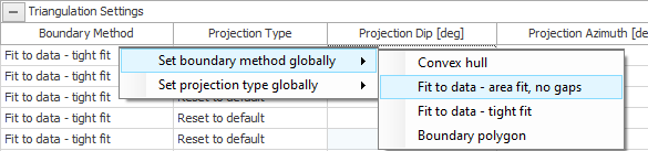
Select the boundary method of your choice from the context menu. click to enlarge
Select the method that you want to use. This method will appear in the Boundary Method column for all surfaces in the table.
Leave the checkboxes checked in the Honor Polyline Segments column to state that all polyline segments will be available again as edges of the generated tri-mesh.
You have now finished the last step of creating a seismic interpretation and assigning surfaces to it. The output surfaces are 2D grids or polyline sets in your seismic interpretation in the JewelExplorer. Optionally, you may have generated fault tri-meshes which you can QC against a seismic backdrop as follows:
- If the assigned surface is a 2D grid, select it in the JewelExplorer or in the 3D View or Seismic View, go toTools > Editing Tools and the 2D Grid editing tools become available in the floating palette. You are then able to remove undesired (interpreted) areas using the 'Remove nodes under line' and the 'Remove node' tools, or, in seismic views, you can use auto-tracking tools to extend/modify the 2D grid.
- If you created one or more tri-meshes you can review them in the 3D View. If the resulting surfaces need to be adjusted, edit the underlying fault interpretations (i.e. the polyline sets) instead of the tri-meshes
For details on how to use the polyline set and 2D grid editing tools, see Structural interpretation of seismic data.
For details on how to use the polylinse set editing tools, see Graphically editing polylines. For more details on how to use the 2D grid editing tools, see Removing nodes from 2D grids.